- Routing
AI route optimization: what it actually saves
Route optimization builds each day's stop sequence from live constraints — vehicle capacity, delivery windows, driver hours, service times and traffic — instead of a planner's spreadsheet. It saves money by cutting miles and by filling vehicles more fully. Savings depend on how much slack your current routes carry, so treat vendor percentages as ranges to test, not promises.
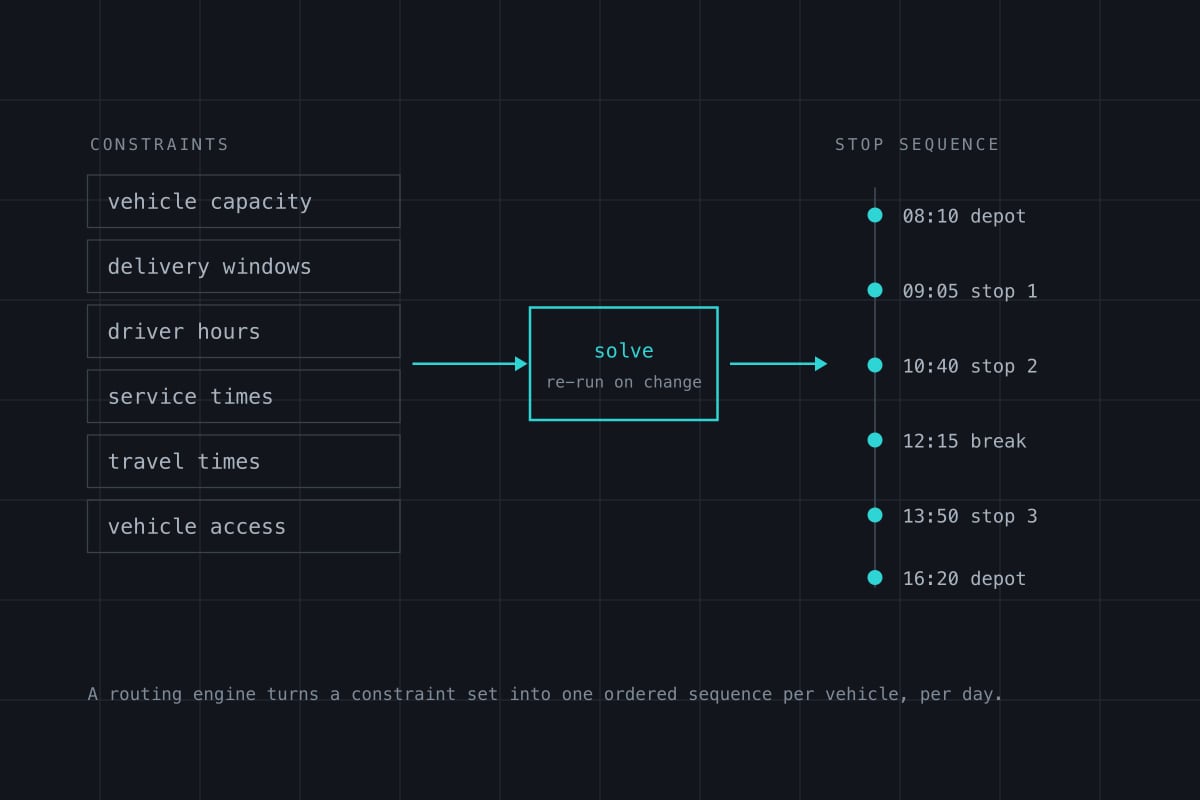
Every dispatcher who has built a day by hand knows the shape of the problem, and it is not the shape the word "route" suggests. You are not looking for a shorter road between two points. You are deciding which stops belong to which vehicle, in what order each vehicle takes them, and whether the day that falls out of those two decisions is legal, deliverable and worth running. The decisions interact, which is why the plan that looks obviously right on a map is so often the one that runs late.
What a routing engine is actually solving
The inputs that decide a sequence are mostly not about distance. Distance is the easy part and it is already solved; what makes routing hard is that every stop carries conditions, and the conditions conflict.
- Capacity. Weight, cube and pallet positions, plus whether the vehicle that can carry the load is also the vehicle that can get a tail lift to the door.
- Time windows. The customer's window, the site's receiving hours, and the hours a residential street will tolerate a box truck at the kerb.
- Driver hours. Federal, and hard. A property-carrying driver may drive 11 hours inside a 14-hour window that opens when they come on duty after 10 consecutive hours off, and may not drive after 8 cumulative hours of driving without a 30-minute interruption[hos]. Weekly the limit is on-duty time, not driving time: 60 hours of it in any 7 consecutive days for a carrier that does not operate every day, or 70 in any 8 for one that does[hos]. Service time at the stop spends that weekly budget without touching the daily driving limit — a real constraint on how a solver packs a week.
- Service time. How long the stop itself takes. This is the input operators get wrong most often, and the one a plan is least able to recover from.
- Travel time, not distance. The same three-mile leg at 08:10 and at 15:40 is two different journeys, and only one of them fits the window.
- Vehicle-to-site fit. Bridge heights, weight-restricted roads, yard access, dock type, whether the site will take a trailer at all.
Put those together and the problem stops being geometric. Twenty stops can be put in order in 20 factorial ways, which is not a number you search through — it is a number you prune. That pruning is the whole job: a solver applies the constraints first to throw away everything illegal or undeliverable, then improves what survives against an objective you chose, usually some weighting of distance, time, overtime risk and vehicle count. Where the "AI" label earns its place is narrow and worth naming: learned estimates of travel time and service time from your own delivery history, feeding the same constrained search. That is a real improvement over a static matrix, and it is a different claim from the one the word usually carries. For the plain definition underneath all of this, see what route optimization means.
Where the money is: miles, and the vehicles they are spread across
Routing pays in two currencies and they are not the same size.
The first is the mile you do not drive. The American Transportation Research Institute puts the industry-average cost of operating a truck in 2025 at $2.336 per mile, and the same cost excluding fuel at $1.854 per mile[atri]. Read the population first: the sectors that release reports margins for are truckload, refrigerated, tank, LTL and flatbed[atri], and it names no parcel or final-mile sector, so for a local delivery fleet these are an order of magnitude rather than your cost — check the report's own population before you treat either as a rate. The difference between the two, $0.482 per mile, is the fuel[atri]. That is the figure a shorter sequence returns to you, and it moves with the pump: the U.S. average on-highway diesel price in the week to 31 August 2026 was $5.599 per gallon[eia], and a fleet's cost per mile tracks it directly.
The second currency is the vehicle you do not send. If a better sequence lets the same work finish on nineteen vehicles instead of twenty, you have not saved fuel on the twentieth — you have saved everything it costs, which on ATRI's numbers is the whole $2.336 for every mile it would otherwise have run[atri]. That is roughly five times the return per mile of the fuel saving alone.
This is why "how much does routing save" is a badly formed question. The honest answer depends on which currency your operation can actually spend. A fleet running near capacity every day, where dropping a vehicle is not on the table, will collect the fuel currency and nothing else. A fleet whose vehicles finish at two in the afternoon has the expensive currency available and usually does not know it. Both are common; they are not the same business case, and a vendor percentage that does not distinguish them is telling you about somebody else's fleet.
Two adjacent lines belong in the same arithmetic, because a routing change moves them and a fuel report will not show it: deadhead miles run empty between the last drop and the yard, and any backhaul load a tighter sequence makes room for.
Sizing the saving on your own numbers
The model below is arithmetic, not evidence. Every row is a number to replace, including the two that carry a citation: those are ATRI over-the-road averages standing in for a delivery fleet they do not describe, and they are the rows the result is most sensitive to. Writing it out makes the shape of the answer visible — which input actually moves the total.
| Line | Value | Basis |
|---|---|---|
| Vehicles | 20 | your fleet |
| Miles per vehicle, per operating day | 90 | your telematics |
| Operating days a year | 250 | your calendar |
| Fleet miles a year | 450,000 | 20 by 90 by 250 |
| Fuel cost a mile | $0.482 | ATRI over-the-road average, 2025 — replace with your own[atri] |
| Fuel spend a year | $216,900 | 450,000 at $0.482 |
| Miles removed by a better sequence | 6% | the number to test, never to assume |
| Fuel returned | $13,014 | 6% of the fuel spend |
| Non-fuel cost a mile | $1.854 | ATRI over-the-road average, 2025 — replace with your own[atri] |
| One vehicle's miles a year | 22,500 | 90 by 250 |
| The twentieth vehicle, excluding fuel | $41,715 | 22,500 at $1.854 |
Read the last two lines against the fuel line. On these inputs, removing six per cent of the miles is worth about a third of what removing one vehicle is worth, and the vehicle line does not require the routes to get shorter at all — only better packed. The ratio is the transferable part, not the dollars: substitute your own two cost-per-mile figures and the ranking holds. That is the sensitivity that matters, and it is the one most business cases get backwards, because fuel is the number on the invoice and the truck is the number on the balance sheet.
Run it again with your own service times and your own day length before you take it anywhere. If the model says the vehicle currency is available to you, the next question is not a percentage — it is whether your customers' windows will let you consolidate at all.
What happens when the day changes
A plan built at 05:30 is a claim about a day that has not happened yet, and the first exception falsifies part of it. What separates a routing system that gets used from one that gets switched off is what it does at 10:40, not what it did at 05:30.
A re-plan is not a fresh solve, and treating it as one is the classic implementation failure. Three things are already fixed by mid-morning and a naive solver does not know it: the stops that have been delivered, the ETA the customer was sent at 07:15, and the part of the driver's 11-hour driving limit that has already been spent[hos]. A re-plan has to inherit all three as constraints, not rediscover them as options.
The failure mode is specific and it has a cause. A re-plan that moves a stop from a driver who is running late to one who is running early looks strictly better on the map and is worse in the yard, because the freight is physically on the first vehicle. Unless the re-plan is restricted to the stops still on the truck it is planning — or unless the operation genuinely supports a mid-route transfer, which almost none do — it emits a sequence nobody can execute. The dispatcher overrides it once, then twice, then stops looking. That is how a routing system ends up live, paid for and ignored.
The useful test to put to any vendor, including this one, is not "does it re-optimise". It is: what does a re-plan treat as immovable, and what does it do with the ETA that has already gone out? Shyftbase runs routing as a module on the same system as billing and warehousing, which is the part that decides whether a re-plan reaches the pick sequence and the invoice or stops at the map. A router that re-sequences the road and leaves the paperwork describing the old plan has moved the reconciliation problem rather than removed it.
What it looks like when it works: a decoupling, not a drop
The most useful published evidence on routing at scale is not a vendor case study. It is a line in an annual report.
In its 2016 Form 10-K, UPS told the Securities and Exchange Commission that in its U.S. domestic package operations, average daily volume and delivery stops rose 4.1% and 4.4% respectively while average daily package miles driven rose 0.2%, and attributed the gap to the deployment of its ORION routing system[ups]. The year before, the same filing reports average daily vehicle miles down 0.4% while package volume rose 1.8%[ups].
Read that carefully, because it is not the claim the vendor slide makes. Almost nothing fell. Stops grew and miles very nearly did not, and that is the actual signature of routing working in a business that is also growing: not a fuel line that drops, but a mile count that stops tracking the stop count.
This has a direct consequence for how you measure your own project, and it is the reason a lot of successful routing deployments get written up as failures. If volume is growing and you set success as a fall in total fuel spend, you will conclude the system did nothing, because the saving was spent absorbing the growth. Measure miles per stop, and measure it against the trend line you were on before, not against last month. If you are not growing, total miles is a fair measure and the arithmetic in the previous section applies directly.
Where this breaks, and what it will not fix
A stated boundary is worth more than another percentage, so here is where the case for this stops.
Routes with no slack in them. A dense urban round already running near capacity, planned for years by someone who knows the streets, has little left to give on sequence. The gain there comes from consolidation and from vehicle count, not from a shorter road.
Sequences you do not control. Where the receiving site dictates its slot and the slots are scattered, the sequence is an output of somebody else's calendar. A solver can tell you what that is costing you, which is genuinely useful in a commercial conversation, but it cannot fix it.
Single-drop full loads. One pickup, one delivery, no sequence to build. The planning gain in linehaul is in load building and backhaul matching, which is a different problem with a different tool.
When the dock is the binding constraint. If vehicles are waiting to load rather than waiting to drive, the road plan is not the thing limiting the day, and a better sequence will simply move the queue.
When the master data is wrong. This is the most common cause of a failed deployment and the least discussed. A plan that assumes eight minutes at a stop that really takes twenty-five collapses before lunch, and it collapses with more confidence than the planner it replaced. Service times, access restrictions and vehicle-to-site fit have to be right before any of the arithmetic above means anything — which usually makes the first month of a routing project a data project.
The cost per mile is borrowed from a different kind of truck. Both cited rates are ATRI's 2025 industry averages, reported across truckload, refrigerated, tank, LTL and flatbed carriers and applied above to a short delivery day. Per-mile cost is fixed cost divided by miles, so a rate drawn from trucks covering several times the annual mileage understates a vehicle-year at that distance, and both headline figures inherit it.
The assumptions in the model. The twenty-vehicle table assumes an even day, a stable customer base and that removing a vehicle removes its cost rather than parking it. If the vehicle stays on the fleet and stays insured, the second currency is not available and only the fuel line moves.
Sources
- [hos] 49 CFR 395.3 — Maximum driving time for property-carrying vehicles — U.S. Office of the Federal Register (eCFR). Accessed 8 September 2026.
- [atri] New ATRI Report Details Accelerating Costs and Low Profitability Despite Cuts — American Transportation Research Institute, 15 July 2026. Accessed 8 September 2026.
- [ups] United Parcel Service, Inc. Form 10-K for the fiscal year ended 31 December 2016 — United Parcel Service, Inc., filed with the U.S. Securities and Exchange Commission, 21 February 2017. Accessed 8 September 2026.
- [eia] Gasoline and Diesel Fuel Update — weekly on-highway diesel prices — U.S. Energy Information Administration, 1 September 2026. Accessed 8 September 2026.